8  Module 1.5: Why Visualize Your Data?

“A picture is worth a thousand words” - this is especially true for data! Plots help us to:

• Explore: Understand the distribution of your traits (e.g., Yield, Height). See relationships between variables. Identify patterns.
• Diagnose: Spot potential problems like outliers (strange values) or unexpected groupings. Check assumptions of statistical models.
• Communicate: Clearly present your findings to colleagues, managers, or in publications.

8.1 Introducing ggplot2: The Grammar of Graphics

R has basic plotting functions, but we will focus on the ggplot2 package, which is part of the tidyverse. It’s extremely powerful and flexible for creating beautiful, publication-quality graphics.

ggplot2 is based on the Grammar of Graphics. The idea is to build plots layer by layer:

1. ggplot() function: Start the plot. You provide:
   • data: The data frame containing your variables.
   • mapping = aes(...): Aesthetic mappings. This tells ggplot how variables in your data map to visual properties of the plot (e.g., map Yield to the y-axis, Height to the x-axis, Variety to color).
2. geom_ functions: Add geometric layers to actually display the data. Examples:
   • geom_point(): Creates a scatter plot.
   • geom_histogram(): Creates a histogram.
   • geom_boxplot(): Creates box-and-whisker plots.
   • geom_line(): Creates lines.
   • geom_bar(): Creates bar charts.
3. Other functions: Add labels (labs()), change themes (theme_bw(), theme_minimal()), split plots into facets (facet_wrap()), customize scales, etc. Each function also allows you to edit aesthetic characteristics such as size, color, etc.

8.2 Let’s Make Some Plots!

First, load the necessary libraries:

# Load necessary libraries
library(ggplot2)
library(dplyr) # Often used with ggplot2 for data prep

Now, let’s create a sample breeding data frame for plotting.

set.seed(123) # for reproducible random numbers
breeding_plot_data <-
  tibble(
    PlotID = paste0("P", 101:120),
    Variety = factor(rep(c("ICARDA_A", "ICARDA_B", "Check_1", "Check_2"), each = 5)),
    Location = factor(rep(c("Baku", "Ganja"), each = 10)),
    Yield = rnorm(20, mean = rep(c(6, 7, 5, 5.5), each = 5), sd = 0.8),
    Height = rnorm(20, mean = rep(c(90, 110, 85, 88), each = 5), sd = 5)
  )

# Take a quick look at the data structure
glimpse(breeding_plot_data)

Rows: 20
Columns: 5
$ PlotID   <chr> "P101", "P102", "P103", "P104", "P105", "P106", "P107", "P108…
$ Variety  <fct> ICARDA_A, ICARDA_A, ICARDA_A, ICARDA_A, ICARDA_A, ICARDA_B, I…
$ Location <fct> Baku, Baku, Baku, Baku, Baku, Baku, Baku, Baku, Baku, Baku, G…
$ Yield    <dbl> 5.551619, 5.815858, 7.246967, 6.056407, 6.103430, 8.372052, 7…
$ Height   <dbl> 84.66088, 88.91013, 84.86998, 86.35554, 86.87480, 101.56653, …

8.2.1 1. Scatter Plot: Relationship between Yield and Height

See if taller plants tend to have higher yield in this dataset.

# 1. ggplot(): data is breeding_plot_data, map Height to x, Yield to y
# 2. geom_point(): Add points layer
# 3. labs() and theme_bw(): Add labels and theme
plot1 <-
  ggplot(data = breeding_plot_data, mapping = aes(x = Height, y = Yield)) +
  geom_point() +
  labs(
    title = "Relationship between Plant Height and Yield",
    x = "Plant Height (cm)",
    y = "Yield (kg/plot)",
    caption = "Sample Data"
  ) +
  theme_bw() # Use a clean black and white theme

# Display the plot
plot1

Relationship between Plant Height and Yield.

Let’s color the points by Variety:

# Map 'color' aesthetic to the Variety column
# Adjust point size and transparency for better visibility
plot2 <-
  ggplot(data = breeding_plot_data, mapping = aes(x = Height, y = Yield, color = Variety)) +
  geom_point(size = 2.5, alpha = 0.8) + # Make points slightly bigger, semi-transparent
  labs(
    title = "Height vs. Yield by Variety",
    x = "Plant Height (cm)",
    y = "Yield (kg/plot)"
  ) +
  theme_minimal() # Use a different theme

# Display the plot
plot2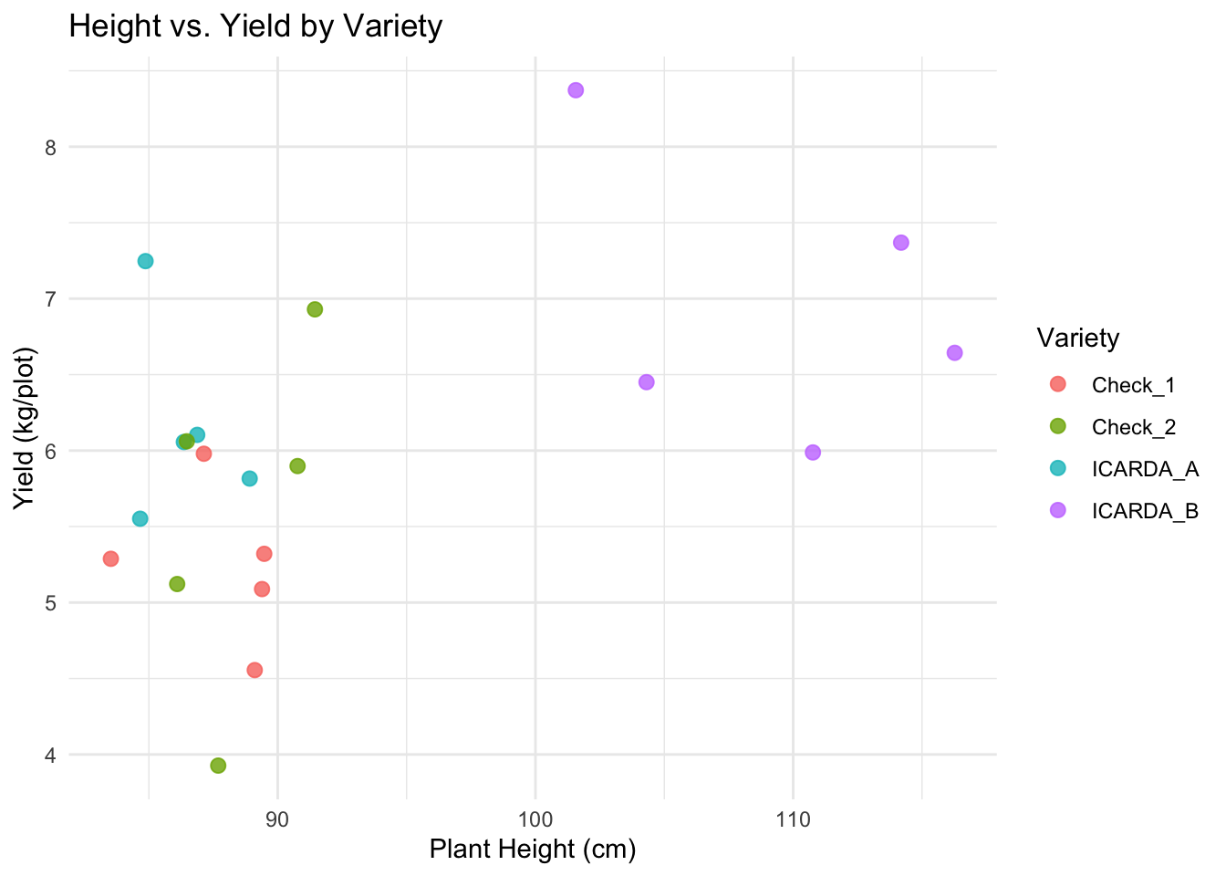

Height vs. Yield by Variety, colored by Variety.

8.2.2 2. Histogram: Distribution of Yield

See the frequency of different yield values.

# 1. ggplot(): data, map Yield to x-axis
# 2. geom_histogram(): Add histogram layer. Adjust 'binwidth' or 'bins'.
# 3. labs() and theme_classic(): Add labels and theme
plot3 <-
  ggplot(data = breeding_plot_data, mapping = aes(x = Yield)) +
  geom_histogram(binwidth = 0.5, fill = "lightblue", color = "black") + # Specify binwidth, fill, and outline color
  labs(
    title = "Distribution of Plot Yields",
    x = "Yield (kg/plot)",
    y = "Frequency (Number of Plots)"
  ) +
  theme_classic()

# Display the plot
plot3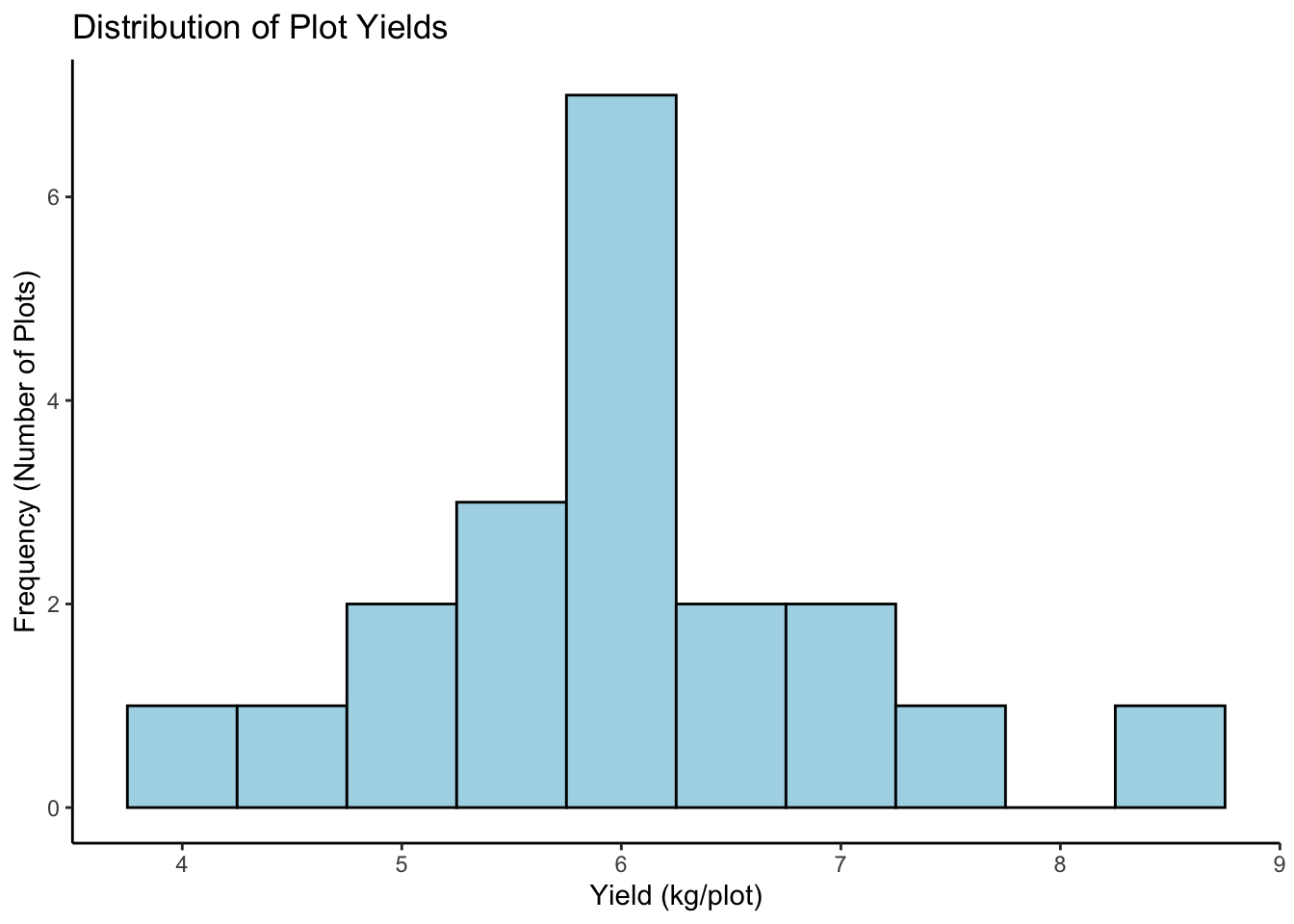

Distribution of Plot Yields.

8.2.3 3. Box Plot: Compare Yield across Locations

Are yields different in Baku vs. Ganja? Box plots are great for comparing distributions across groups.

# 1. ggplot(): data, map Location (categorical) to x, Yield (numeric) to y
# 2. geom_boxplot(): Add boxplot layer. Map 'fill' to Location for color.
# 3. labs() and theme_light(): Add labels and theme
# 4. theme(): Customize theme elements (e.g., remove legend)
plot4 <-
  ggplot(data = breeding_plot_data, mapping = aes(x = Location, y = Yield, fill = Location)) +
  geom_boxplot() +
  labs(
    title = "Yield Comparison by Location",
    x = "Location",
    y = "Yield (kg/plot)"
  ) +
  theme_light() +
  theme(legend.position = "none") # Hide legend if coloring is obvious from x-axis

# Display the plot
plot4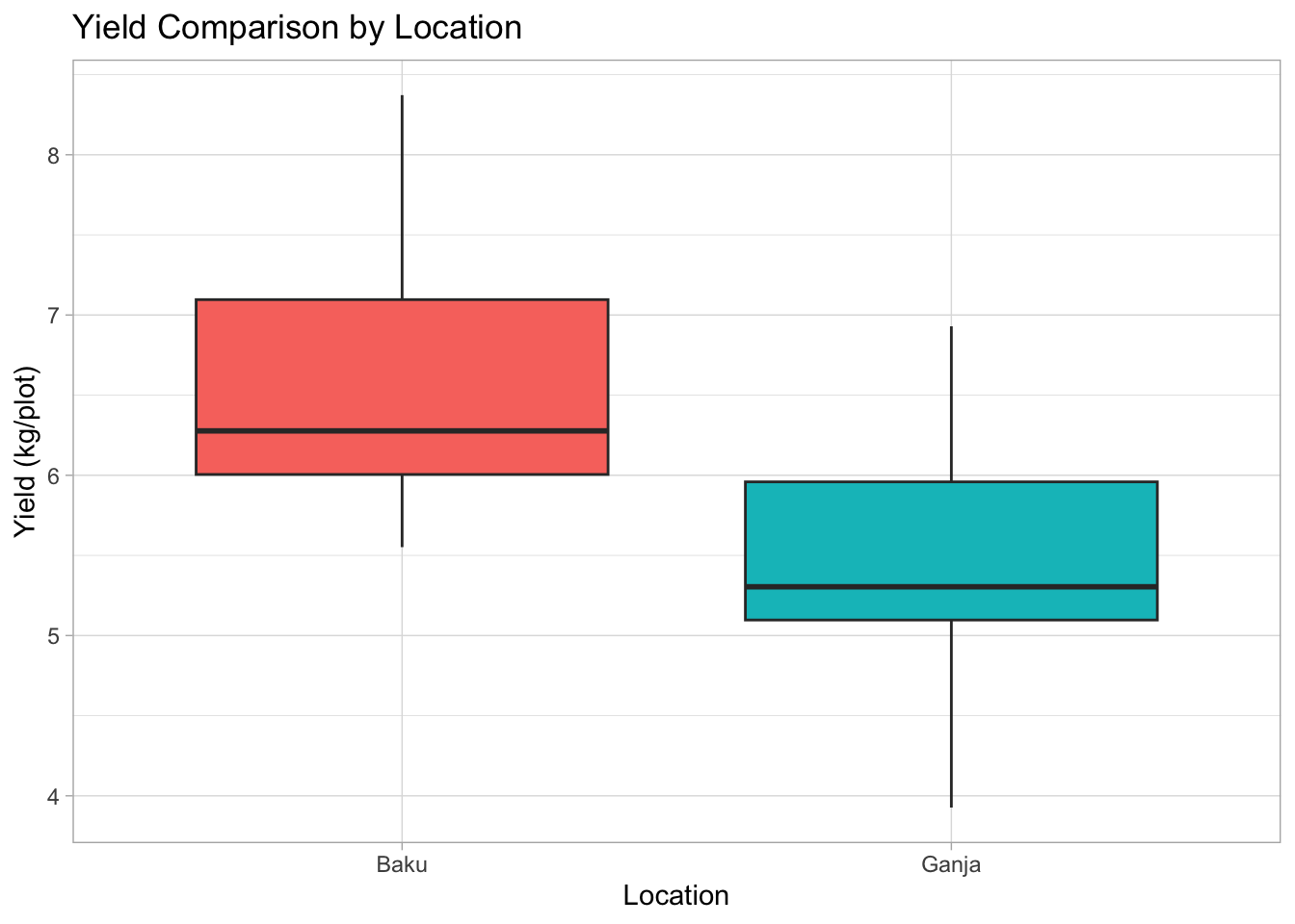

Yield Comparison by Location.

Box plot anatomy: The box shows the interquartile range (IQR, middle 50% of data), the line inside is the median, whiskers extend typically 1.5*IQR, points beyond are potential outliers.

8.3 Saving Your Plots

Use the ggsave() function after you’ve created a ggplot object (like plot1, plot2, etc.).

# Make sure the 'output/figures' directory exists
# The 'recursive = TRUE' creates parent directories if needed
output_dir <- "output/figures"
if (!dir.exists(output_dir)) {
  dir.create(output_dir, recursive = TRUE)
}

# Save the height vs yield scatter plot (plot2)
ggsave(
  filename = file.path(output_dir, "height_yield_scatter.png"), # Use file.path for robust paths
  plot = plot2,                               # The plot object to save
  width = 7,                                  # Width in inches
  height = 5,                                 # Height in inches
  dpi = 300                                   # Resolution (dots per inch)
)

# You can save in other formats too, like PDF:
# ggsave(
#   filename = file.path(output_dir, "yield_distribution.pdf"),
#   plot = plot3,
#   width = 6,
#   height = 4
# )

8.4 Exercise

Create a box plot comparing Plant Height (Height) across the different Varieties (Variety) in the breeding_plot_data. Save the plot as a PNG file named height_variety_boxplot.png in the output/figures directory.

# Exercise: Box plot comparing Plant Height across Varieties
plot5 <-
  ggplot(data = breeding_plot_data, mapping = aes(x = Variety, y = Height, fill = Variety)) +
  geom_boxplot() +
  labs(
    title = "Plant Height Comparison by Variety",
    x = "Variety",
    y = "Plant Height (cm)"
   ) +
  theme_light() +
  theme(legend.position = "none")

# Display the new plot
plot5

Plant Height Comparison by Variety.

# Ensure output directory exists
output_dir <- "output/figures"
if (!dir.exists(output_dir)) {
  dir.create(output_dir, recursive = TRUE)
}

# Save the box plot as a PNG file
ggsave(
  filename = file.path(output_dir, "height_variety_boxplot.png"),
  plot = plot5,
  width = 7,
  height = 5,
  dpi = 300
)